Kilofarad

I know what kilo means. I know what farad means. But even so, I never thought I’d have a use for the word kilofarad — let alone have one on my desk.

One kilofarad (two 500F caps in parallel). Hard to believe, but there it is.

The farad, named after Michael Faraday, is the SI unit of capacitance. It is equal to one coulomb of charge per volt. One coulomb is equivalent to one amp-second: one amp of current flowing for one second transfers one coulomb of charge.

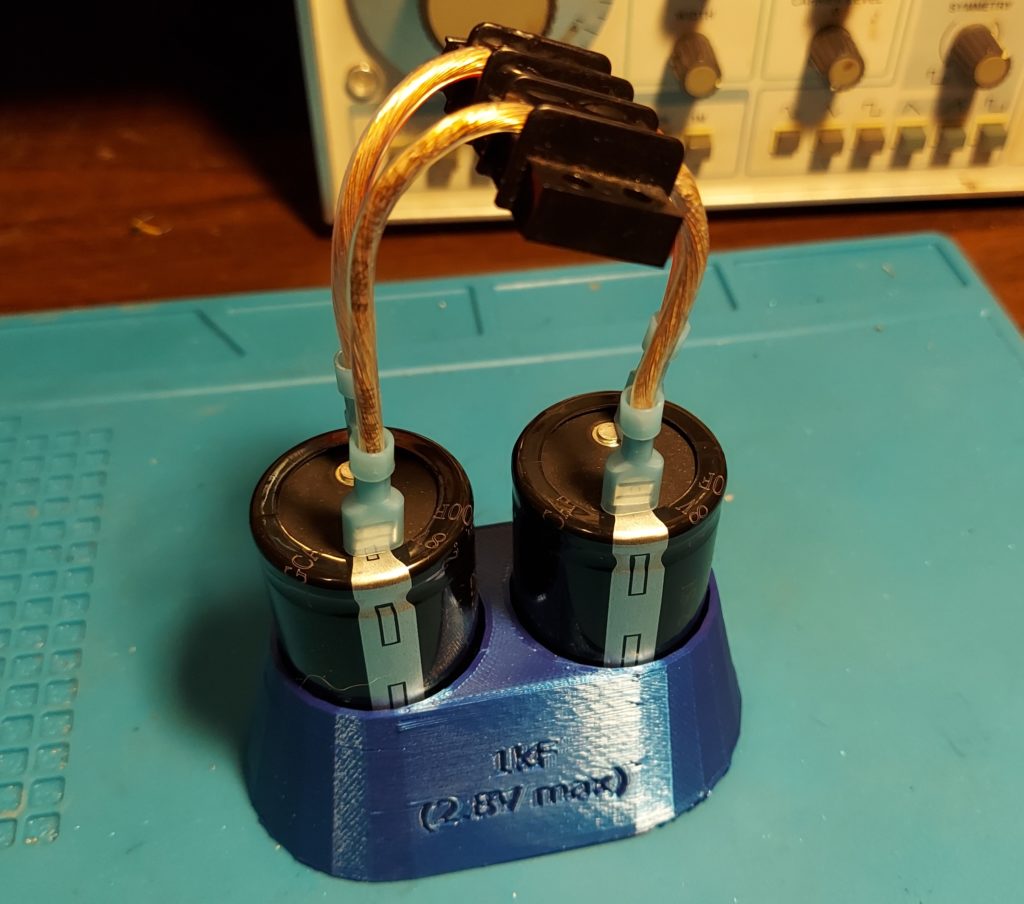
This suggests an experiment: Charge a parallel pair of 500F capacitors (a kilofarad compound capacitor) at a constant 1A, as measured by a trusted DVM. Put another meter in DC voltage mode across the capacitor, and log the rate of change of voltage. (One kilofarad should be one millivolt per coulomb of charge, so we can use voltage as a “gas gauge” for how much charge is stored.)

For a textbook 1kF capacitor charged at a constant 1.0 amps, voltage should rise at 1mV per second, or 3.6V per hour. Since the power supply will have to provide some overvoltage in order to make up for any system losses and keep 1A flowing, this experiment has to be carefully monitored to avoid overcharging the capacitors.

It’s not that they’re particularly expensive. It’s that a 1kF capacitor, charged to 2.7V, stores some 3.6kJ of energy. That’s enough to lift even my 100kg posterior some 3.33m, or almost 11 feet, straight up. To imagine what a failed cap would be like, imagine sitting on an ejection chair powered by an explosive charge powerful enough to launch a large adult ten feet in the air. That’s how much energy is in there — at only 2.7V!
(“Danger: Low Voltage”…??)

Charging at a constant 1A (kept generally within 1mA) resulted in the following voltage/charge curve. (Upon reaching 2.75V, the power supply was disconnected and the capacitors allowed to self-discharge. Effective capacitance was not measured past that point.) Interestingly, voltage rose more slowly with increasing charge. The orange curve on the chart shows effective capacitance to each point. When charged to at least 1.1V or so, the two 500F capacitors do seem to make a one-kilofarad pair.

…At least, if there has been no significant loss of charge. Measuring that will need either a controlled-current load, or simultaneous monitoring of both voltage and current, since any simple resistive load will likely experience significant changes in resistance as it heats up.

Voltage (blue, volts) and effective capacitance (orange, kilofarads)
Posted in Analog, Components, Electronics, Fundamentals, Mad Science, Reviews, Science, Toys | Tagged , , , , , , , , , , , , , | Leave a comment

Mini Museum: TRS-80 Model 200

A Tandy 200 — essentially, a Model 100 with 2x the display area and a clamshell case.

The “Tandy 200” (Tandy had by then dropped the TRS-80 label) is an upgraded TRS-80 Model 100. The most noticeable upgrade, of course, is the new clamshell display, with twice the display area as on the Model 100. Better cursor keys are another improvement.

The -200 also has banked memory. Presumably for backwards compatibility, the system memory is limited to 32kB, but the -200 can access three (?) memory banks of 32kB each, by switching between them. Kind of like having three different computers in one, I guess?

The processor in the Model 100, -102, and Tandy 200 is an Intel 8085. Despite the similarity in number to the Intel 8088 powering the original IBM PC, the 8085 is essentially an 8080 with a few tweaks and a single-rail 5V power supply to make integration easier. It has more in common with Z80 machines like the Timex/Sinclair 1000 than it does with x86 machines.

While the Tandy 200 is an improvement over the Model 100, it turned out to not be as popular. Even the Model 102 — really just an updated 100 — sold more units. The reasons given were price (the larger display no doubt cost more) and size. While the -200 is significantly thicker and heavier than a Model 100, the laptops of just a few years later would make it almost look like a pocket computer. (IBM PC Convertible with optional printer module, we’re looking at you.)

While I don’t have nearly as much personal history with this one as with my Model 100 (which was my main computer for a few years until I built the ‘486), it’s interesting to see the differences.

I should put an ESP32 on the RS232 port as a dongle and let it browse the Web via lynx…

Posted in BASIC, Drexel, Mini Museum, Nostalgia, Tools | Leave a comment

Mini Museum: TRS-80 Model 100

A Model 100 laptop, from the early 1980s.
(I’d update its date to 2023, but it wouldn’t believe me.)

The TRS-80 Model 100 was one of the first popular “laptop” style computers. Offered for sale in 1983, it was a revolutionary device. Users could choose from built-in BASIC as well as rudimentary word processor, scheduler, address book, and terminal apps. It spoke a surprisingly mainstream dialect of BASIC for the day — a lot like IBM BASICA available on the first DOS machines.

Power was provided from either a wall-wart adapter or car adapter, or four AA batteries, which would actually run the machine for many hours. (Radio Shack claimed about 20 hours runtime, and I found that believable.) A memory backup battery was also provided, so if the AA batteries ran out or were removed, you didn’t lose your data.

Program storage was either the 22KB of battery-backed-up memory, shared between program storage and RAM, or “bulk storage” via audio transfer to cassette tape. There was an obscure “Disk/Video Adapter” (the size of a small PC) that could connect to the Model 100 via the expansion port on the bottom, and allowed it to read and write low-density 5.25″ diskettes. It was more reliable than the tape option — but then again, so was almost literally anything else.

There was a built-in direct-connect modem, and with the addition of a phone adapter cable, the Model 100 could dial in to a server. Dial up BBSes (Bulletin Board Systems) were the “Internet” of the day; most of the menus were designed for full-size CRT terminals and didn’t look good on the Model 100’s small LCD screen — but the “killer app” for these was the ability for journalists to call in and directly upload draft articles straight from on-assignment locations, using only a phone line. (The alternative tech was to use a fax machine and have someone re-type the article.)

One thing that the Model 100 was great at was RS232 serial communication. Back in the day when 9,600 baud was the standard that all the cool, high-speed kids used, the ability to do serial comms at any speed from 75 baud to 19,200 baud was amazing. And the Model 100 could do this with 6, 7, or 8 data bits, one or two stop bits, with parity bit options of Mark, Space, Even, Odd, or None. (That’s literally every option mathematically possible, for those keeping score.) If it had a serial port, the M100 could talk to it.

One serial device that I got it to talk to was an old LORAN-C receiver that I picked up for cheap at a hamfest. LORAN-C was a wide-area navigation system from back before GPS and friends were available to non-military users. LORAN (short for LOng-RAnge Navigation) used time/phase differences in groundwave signals sent from sites around the US to determine the user’s position. Finding the time difference between two sites resulted in a hyperbolic line of location. With two (or ideally more) pairs of stations, the position could be determined by the intersection of these positions.

The Model 100’s BASIC turned out to be fast enough to listen to the data provided at NEMA 4800 baud from the LORAN, compress it using a keyframe-plus-deltas scheme I came up with, and store it in its memory. 22KB of memory — not enough for a modern app’s icon — was enough to record some eight hours of position data, with a latitude/longitude fix every six seconds (which was all the LORAN would do.)

I used it to track position data on trips between home (northern VA) and college (Norfolk). On a whim, I did a complete cloverleaf interchange tour on one trip home — taking each of the four 270-degree ramps and continuing on in the original direction. When I got to school and downloaded and plotted the data, the cloverleaf was visible, if somewhat distorted (even driving slowly, a car moves quite some distance in six seconds.)

The 1980s may not have had VR, ChatGPT, or even the Internet as we know it — but we did a lot with almost nothing.

Posted in BASIC, Drexel, Mini Museum, Nostalgia, Tools, Toys | Leave a comment

Components: Inductors

Various inductors (chokes and transformers). Ruler and transit token for scale.

An inductor is probably the simplest electronic component. It is literally a wire, bent into a coil around a core of either air or another substance. Although all real inductors have some resistance (unless made of superconductors), inductors’ usefulness results from their electromagnetic properties — both as electromagnets and in electronic circuits.

Just as a resistor has a characteristic law — Ohm’s Law — that it follows, inductors follow a similar law. (V = L*di/dt) The difference is, inductors develop a voltage proportional to the change in current per unit of time — not the flow of current itself. This property is at the heart of many interesting, useful circuits that make use of inductors:

  • Chokes: Most simply, inductors are used to block high-frequency signals and pass lower-frequency ones. So a RL filter, with the inductor in series, would be a low-pass filter. With the inductor in parallel with the load, it would be a high-pass filter.
  • Resonant circuits: An inductor/capacitor pair can form a resonant circuit, suitable for tuning in radio signals of a particular frequency, or generating AC signals as part of an oscillator.
  • Voltage multiplication: Inductors are often used as the energy-storage elements of switched-mode (buck and/or boost) power supplies. If current flowing through an inductor is suddenly blocked, a high voltage appears across the inductor, which can be collected in a capacitor.
  • Transformers: Two magnetically-coupled coils can convert high voltage to high current or vice-versa.

Basic model

The characteristic equation for inductors is V = L*di/dt. Voltage across the inductor is proportional to its inductance in henries, times the time derivative of current (in amps per second, which sounds like a natural unit, but measures rate of change of the flow of charge.)

So, inductors oppose changes in current flow. The voltage across an inductor, by Lenz’s Law, is in the polarity which will oppose the change in current flow. If no current is flowing, the voltage will oppose current flow. If the current is decreasing, the energy in the inductor will act to keep the current flowing.

At DC, inductors are simply wire, and have resistance but no reactance, since di/dt is zero. With AC, reactance is proportional to frequency — Xc = 2*pi*f*L.

Posted in Components, Electronics | Tagged , , , , , , | Leave a comment