I hope the designer got recognized for this one, because it’s really clever.
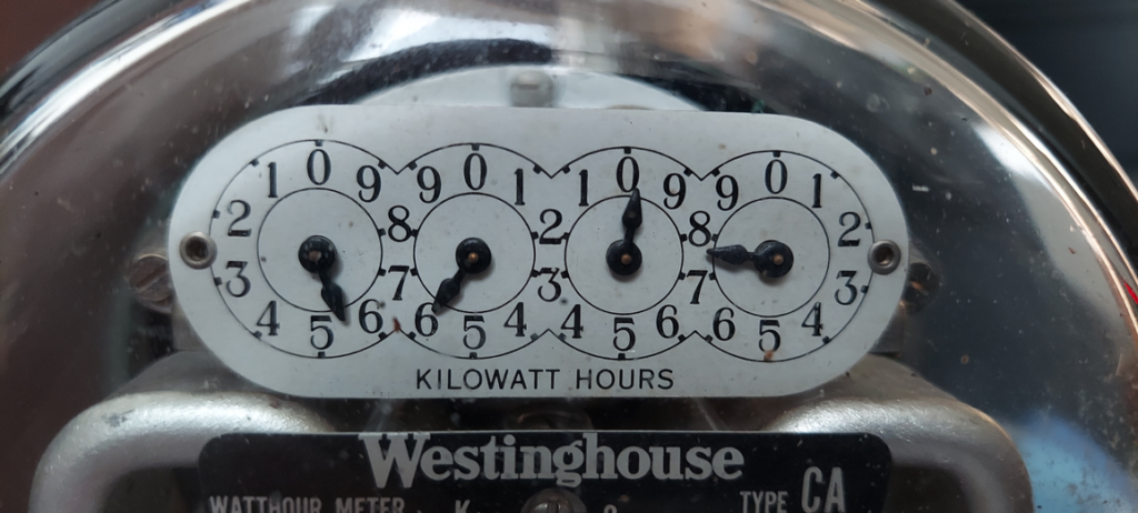
The readout dials of a Westinghouse Type CA watt-hour meter
On a recent trip to the frozen Northlands, I came across a Westinghouse kilowatt-hour meter and picked it up to use in classroom discussions about power and energy.
Looking more closely at it reveals a neat design quirk — the 2nd and 4th indicators move counterclockwise, and so (with reversed scales) can share two digits with each neighbor.
There seems to be enough space in the meter that this wouldn’t be necessary — but perhaps the design was originally from a smaller meter. Or maybe this was just an engineer having fun.
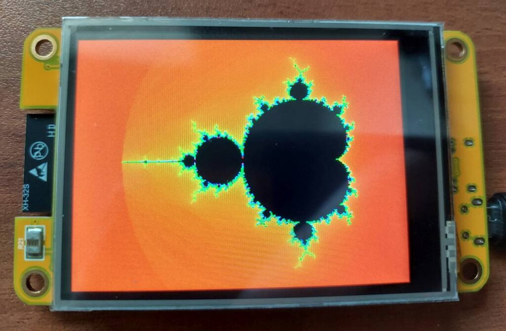
Is this coding? It sure doesn’t seem like it, but it’s sure faster than the old way!
A working zero-shot vibe-coded Mandelbrot zoomer. This was written entirely by GPT-OSS-20B from a single prompt, with no human-contributed code.
Since 2022 or so, we’ve learned that (since programming is at least partially a language-based task) large, multi-billion-dollar LLMs can often produce useful, working code. But we’re now getting to the point where even open-source language models that can run on consumer hardware can do useful coding work, at least if properly prepared.
I recently learned about a useful new ESP32 form factor that everybody seems to be calling the “CYD” (for “Cheap Yellow Display“.) It has all of the usual ESP32 goodies — a dual-core processor, 240MHz clock speed, WiFi, Bluetooth, and so on — plus a 320×240 resistive touchscreen display. It would make a nice modern thermostat or data readout or whatever.
When I work with new hardware or new languages, one of the first familiarization tasks I usually start with is to write a Mandelbrot viewer for it. 320×240 isn’t exactly High Definition, but with 16-bit color, it’s starting to be useful for graphical applications like this.
Instead of writing the Mandelbrot zoomer myself (I’m already familiar with Bodmer’s excellent tft_eSPI library), I decided to see how well GPT-OSS-20B would do with the task. Since local models may or may not have working Internet search capability, I decided to give it a primer. I asked GPT5.2 to write a simple demo sketch that listened for touch sensor input and then drew a green dot at that location, and also provided (in comments) syntax for other library functions. Adding this sketch into the prompt would show a local LLM how the graphics and touchscreen functions work, so they could be incorporated into new code. (After all, it’s a lot more reasonable to expect a model to know C than to be familiar with specific libraries.)
Here is the complete prompt (including Arduino skeleton sketch from GPT5.2) that I provided:
The following is an example Arduino sketch for an ESP32-based “CYD” dev board with a 320×240 pixel touchscreen display. Please create a Mandelbrot Set viewer with a touchscreen interface, using this exact board hardware setup as defined in the “BOARD-SPECIFIC CONSTANTS” section. Various methods for drawing to the screen and reading touch inputs are demonstrated and/or described in the comments. Use these functions to implement a Mandelbrot Set viewer. On reset, start with a view of the whole Set, zoomed appropriately. Once the Set is drawn and a point on the screen is touched, zoom in at a factor of 2.0 (in both x and y), centered on that point. Start with 100 iterations (settable by parameter) and increase as needed. Choose an appropriate color map that will be visible at high and low zoom levels. Use Float for the first 16 zooms, and Double thereafter. Track all position variables as type double. Thanks.
[skeleton Arduino sketch pasted into prompt; file available below]
The gpt-oss-20b model, running under Ollama with a 64k token context window, took about an hour to think about the problem. At one point, I was concerned that it was getting stuck in a loop (it went on and on for dozens of lines about “Now I need to think about X” and “Now I need to think about Y” — some of which made more sense than others. I decided to go watch some YouTube videos and wait to see what happened. After an hour or so, it finished and produced a plausible-looking sketch. I copied and pasted it into the Arduino IDE, hit Upload and waited.
It worked. I didn’t have to change anything. The touch inputs work correctly, the images are correct, and even the color map is appropriately-chosen and works at multiple zoom levels.
This is as big a change as going from machine code to assembly, or from assembly to higher-level languages. Maybe even more profound. We’re at the very least going to see the barrier to entry for writing code effectively removed, allowing anyone to code, and allowing existing engineers to focus on higher-level aspects of design.
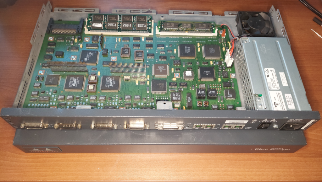
“Well, that takes a lot of the mystique out of Cisco routers…” –Frank Gentges, AK4R (upon seeing one opened up)
A Cisco 2500 router, resting on its removed cover to show the internals.
At one point, probably around the year 2000, it was said that every email (and anything else sent over the Internet) went through one or more Cisco routers. I believe it, at least given the market dominance Cisco enjoyed back in the early Internet days. No doubt, many exabytes of data have flowed through these Internet traffic-control devices.
IP routers are central to packet-switched networks. Working with routing protocols such as RIP and OSPF, they examine the addresses and subnet masks of incoming IP packets, and route those along to the next step. They would typically be paired with a CSU/DSU and connected to a 1.544 Mbit/sec T1 link (which was quite speedy for the time, but quickly got eclipsed once cable modems and fiber-to-the-home became popular. (Gigabit fiber is reasonably common in urban areas, today.)
Although the 2500 is (literally) a museum piece today — its 10BaseT Ethernet connection would be a huge bottleneck even for home Internet connections — the same important job is still being handled by thousands of similar, higher-speed devices. Packet-switched networks (of which the Internet is the poster-child example) do not create persistent electrical connections between nodes which need to communicate with each other. Instead, data is grouped into packets, which are routed node-to-node until they get to their destination.
(This particular router was pulled from service because it developed a problem with its persistent memory, and therefore won’t remember any settings. The company I was contracting for said to keep it.)
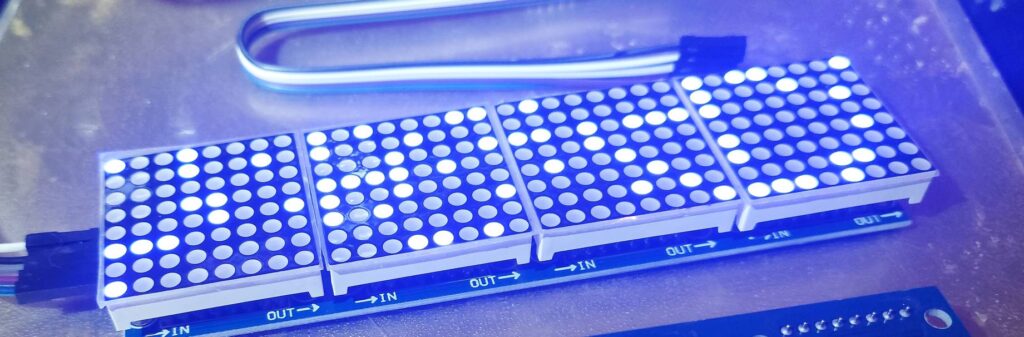
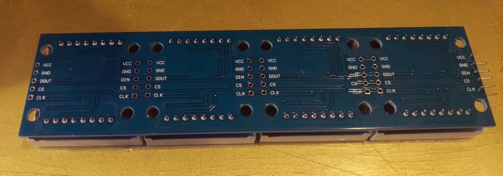
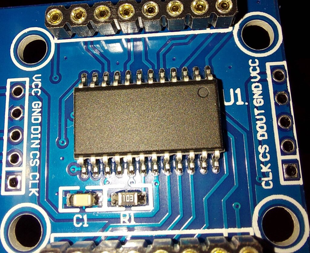
Specialty chips like the MAX7219 can make visually-striking devices easier to work with. The ‘7219 is designed to drive an 8×8 matrix of LEDs, from a single SPI input. Additional modules can be easily added to the chain, allowing the creation of larger displays. A few helper C functions fold the pixels into the usual rectangular shape even if they’re not wired that way. With the SPI interface, updates are fast — at least several dozen Hz for four modules (32×8).
Four blue 8×8 LED modules. (They’re blue, not pale-blue or white — but even the lowest brightness overpowers the camera.)Each module sends excess data on to the next one. The only limit (other than supply current, which could be supplied) is update time.
Weirdly, even though the modules are sold as (and work as) MAX7219 chips, the ICs themselves seem to have had any identifying markings removed. (The original seller photos show both Maxim-branded (now part of Analog Devices) as well as the anonymous chips.)
The product listing says it’s a MAX7219. It works like one. Why the obfuscation?
A basic Arduino sketch (tested on ESP32) is up on GitHub. I’ll probably add digits next, if there isn’t a library already out there, suitable for these. They’d make a good compass display for the Santana.
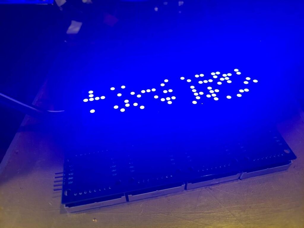
Just don’t try to take a picture of them without strong lighting…
This isn’t how it looks IRL either, but it gives you an idea of the level of blue. At low brightness.